Elastic Functional Principal Component Analysis

After we have aligned our data we can compute functional principal component analysis (fPCA) on the aligned data, warping functions, and jointly

import fdasrsf as fs
import numpy as np

We will load in our example data again and compute the alignment

data = np.load('../../bin/simu_data.npz')
time = data['arr_1']
f = data['arr_0']
obj = fs.fdawarp(f,time)
obj.srsf_align(parallel=True)

Initializing...
Compute Karcher Mean of 21 function in SRSF space...
updating step: r=1
updating step: r=2

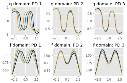
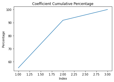
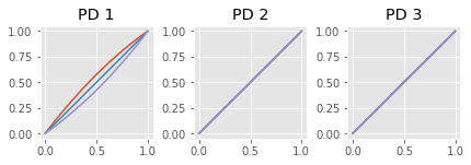
Vertical fPCA

We will first compute fPCA on the aligned functions, by constructing the object and computing the PCA for the number of components, default=3)

vpca = fs.fdavpca(obj)
vpca.calc_fpca(no=3)

We then can plot the principal directions

vpca.plot()

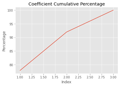
Horizontal fPCA

We can then compute PCA on the set of warping functions

hpca = fs.fdahpca(obj)
hpca.calc_fpca(no=3)

We then can plot the principal directions

hpca.plot()

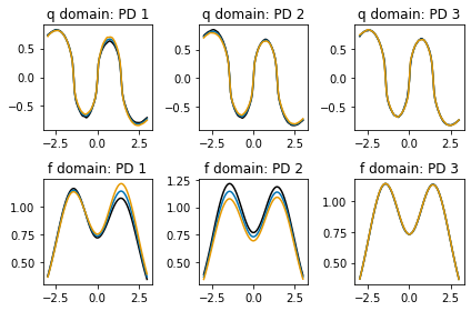
Joint fPCA

We can also compute the fPCA on jointly on the phase/amplitude space if we feel there is correlation between the variabilities

jpca = fs.fdajpca(obj)
jpca.calc_fpca(no=3)

We then can plot the principal directions

jpca.plot()