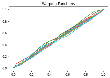
Elastic Curve Alignment#
Otherwise known as time warping in the literature is at the center of elastic functional data analysis. Here our goal is to separate out the horizontal and vertical variability of the open/closed curves
[1]:
import fdasrsf as fs
import numpy as np
Load in our example data
[2]:
data = np.load('../../bin/MPEG7.npz',allow_pickle=True)
Xdata = data['Xdata']
curve = Xdata[0,1]
n,M = curve.shape
K = Xdata.shape[1]

beta = np.zeros((n,M,K))
for i in range(0,K):
    beta[:,:,i] = Xdata[0,i]
We will then construct the fdacurve object
[3]:
obj = fs.fdacurve(beta,N=M)
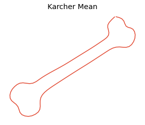
We then will compute karcher mean of the curves
[4]:
obj.karcher_mean()
Computing Karcher Mean of 20 curves in SRVF space..
updating step: 1
updating step: 2
updating step: 3
updating step: 4
updating step: 5
updating step: 6
updating step: 7
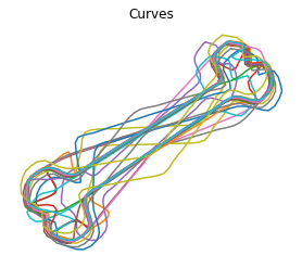
We then can align the curves to the karcher mean
[5]:
obj.srvf_align(rotation=False)
Plot the results
[6]:
obj.plot()
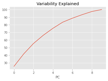
Shape PCA#
We then can compute the Karcher covariance and compute the shape pca
[7]:
obj.karcher_cov()
obj.shape_pca()
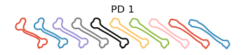
Plot the principal directions
[8]:
obj.plot_pca()